The Loss Surface of Deep and Wide Neural Networks

ICML 2017, 논문링크 : https://arxiv.org/abs/1704.08045

• 저자 : Quynh Nguyen, Matthias Hein

• 초록 (Abstract)

While the optimization problem behind deep neural networks is highly non-convex, it is frequently observed in practice that training deep networks seems possible without getting stuck in suboptimal points. It has been argued that this is the case as all local minima are close to being globally optimal. We show that this is (almost) true, in fact almost all local minima are globally optimal, for a fully connected network with squared loss and analytic activation function given that the number of hidden units of one layer of the network is larger than the number of training points and the network structure from this layer on is pyramidal.

• 요약 (Summary)
  • 딥러닝 학습은 highly non-convex optimization 문제이지만 suboptimal local minima 에 잘 빠지지 않음. 이에 대한 이론적인 설명은 아직 미비함
  • 이 논문에선 레이어의 수가 학습데이터보다 훨씬 많은 상황(Overspecification) 에서 local minima 는 대부분 global optimal 임을 보임
  • Sparse connectivity 를 가지는 네트워크는 위 논문에서 다루지 못함
• 기호 (Notation)
  • \( N \) : 학습 샘플 수
  • \( d \) : Input 의 dimension, \( m \) : Output 의 class 수
  • \( X = [x_{1},\ldots, x_{N}]^{T}\in\mathbb{R}^{N\times d} \) : Input 행렬
  • \( Y = [y_{1},\ldots, y_{N}]^{T}\in\mathbb{R}^{N\times m} \) : Output 행렬
  • \( L \) : Fully-connected feed-forward network 의 레이어 수
  • \( n_{k} \) : \( k \) 번째 레이어의 hidden-unit 수
  • \( \mathcal{W}:=\mathbb{R}^{d\times n_{1}}\times \cdots \times \mathbb{R}^{n_{k-1}\times n_{k}}\times\cdots\times\mathbb{R}^{n_{L-1}\times n_{L}} \) : Weight 행렬의 집합
  • \( (W_{k})_{k=1}^{L}\in\mathcal{W} \) : Weight 행렬
  • \( \mathcal{B} := \mathbb{R}^{n_{1}}\times \cdots \times \mathbb{R}^{n_{L}}\) : Bias 벡터의 집합
  • \( (b_{k})_{k=1}^{L}\in\mathcal{B} \) : Bias 벡터
  • \( \mathcal{P} = \mathcal{W}\times\mathcal{B} \) : 네트워크 패러미터 공간
  • \( [a] := \{1,2,\ldots, a\} \) : 1 부터 정수 \( a \) 까지의 집합
  • \( [a,b] := [b] \setminus [a-1] \) : 정수 \( a \) 부터 정수 \( b \) 까지의 집합
  • \( \sigma : \mathbb{R} \to \mathbb{R} \) : activation 함수 (\( C^{1} \) 조건 필요로 함)
  • \( f_{k}, g_{k} : \mathbb{R}^{d} \to \mathbb{R}^{n_{k}} \) : Input 공간에서 \( k \) 번째 레이어의 feature 공간으로 다음과 같이 매핑하는 함수 :

• • \( F_{k} = [f_{k}(x_{1}),f_{k}(x_{2}),\ldots, f_{k}(x_{N})]^{T}\in\mathbb{R}^{N\times n_{k}} \) : 모든 학습데이터에 대한 \( f_{k} \) 의 값행렬
  • \( G_{k} = [g_{k}(x_{1}),g_{k}(x_{2}),\ldots, g_{k}(x_{N})]^{T}\in\mathbb{R}^{N\times n_{k}} \) : 모든 학습데이터에 대한 \( g_{k} \) 의 값행렬
  • \( \ell :\mathbb{R} \to \mathbb{R} \) : Loss 함수
  • \( \Phi : \mathcal{P}\to\mathbb{R} \) : 네트워크의 Final objective

• 이 논문에선 식 (1) 의 minimum 이 달성되었다고 가정함

Assumption 3.2

1. 학습데이터가 모두 다름. 즉, 모든 \( i\neq j \) 에 대해 \( x_{i}\neq x_{j}\)
2. \( \sigma \) 가 해석적(analytic), 강단조증가(strictly monotonically increasing) 여야 함. 더불어서 유계(bounded) 이거나 선형함수보다 증가속도가 빠르면 안 됌
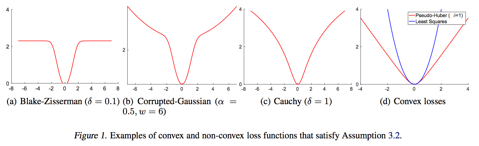
3. Loss 함수가 \( \ell\in C^{2}(\mathbb{R}) \) 이고 \( \ell’(a) = 0 \) 이면 \( a \) 에서 최소값을 가져야 함

• Assumption 의 2번 가정은 대부분의 activation 함수들이 만족함
• \( L_{2} \) - loss 의 경우 ( \( \ell(a) = a^{2} \) ) 3번 가정을 충족
• \( L_{2} \) - loss 이외에 아래와 같은 loss 함수들도 3번 가정을 충족

Theorem 3.4 Assumption 3.2 하에서, 학습데이터들이 선형적으로 독립(linearly independent) 이라고 하자. 이 때 식 (1) 의 모든 critical point \( (W_{l},b_{l})_{l=1}^{L} \) 들은 Weight 행렬들이 full-column rank 를 가질 때 global minimum 이다

• 위 정리에서 학습데이터가 선형적으로 독립이라는 가정은 \( N \leq d+1 \) 을 뜻하므로 매우 강한 제약이다
• 학습데이터가 아니라 Hidden 레이어의 변수들이 충분히 많다면 위 가정을 대체할 수 있다

Theorem 3.8 Assumption 3.2 하에서, 어떤 \( k\in [L-1] \) 에 대해 \( n_{k} \geq N-1 \) 을 만족한다고 가정하자.